
8 Algorithmes de Machine Learning expliqués en Langage Humain

Ce qu'on appelle Machine Learning ou Apprentissage automatique n'est autre que la rencontre des statistiques avec la puissance de calcul disponible aujourd'hui (mémoire, processeurs, cartes graphiques).Ce domaine a pris toute son importance en raison de la révolution digitale des entreprises qui a conduit à la production de données massives de différentes formes et types, à des rythmes sans cesse en augmentation : le Big Data.Sur un plan purement mathématique la plupart des algorithmes utilisés ont déjà plusieurs dizaines d'années. Dans cet article je vous expliquerai le fonctionnement de 8 algorithmes d'apprentissage automatique et ce dans les termes les plus simples possibles.
1. Quelques grands concepts avant d'aborder les algorithmes
A. Classification ou Prédiction ?
Classification
Attribuer une classe / catégorie à chacune des observations d'un jeu de données est une classification. Se fait à posteriori, une fois les données récupérées.Exemple : classification des raisons de visite de consommateurs en magasin dans le but de créer une campagne marketing hyperpersonnalisée.
Prédiction
Une prédiction se fait sur une nouvelle observation. Lorsqu'il s'agit d'une variable numérique (continue) on parle de régression.Exemple : prédiction d'un AVC d'après les données d'un électro-cardiogramme.
B. Apprentissage supervisé et non supervisé
Supervisé
Vous disposez déjà d'étiquettes sur des données historiques et vous cherchez à classifier des nouvelles données. Le nombre de classes est connu.Exemple : en botanique vous avez effectué des mesures (longueur de la tige, des pétales, …) sur 100 plantes de 3 espèces différentes. Chacune des mesures est étiquetée de l'espèce de la plante. Vous souhaitez construire un modèle qui saura automatique dire à quelle espèce une nouvelle plante appartient d'après le même type de mesures.
Non Supervisé
Au contraire, en apprentissage non supervisé, vous n'avez pas d’étiquettes, pas de classes prédéfinies. Vous souhaitez repérer des motifs communs afin de constituer des groupes homogènes à partir de vos observations.Exemple : Vous souhaitez classifier vos clients d'après leur historique de navigation sur votre site internet mais vous n'avez pas constitué de groupes à priori et êtes dans une démarche exploratoire pour voir quels seraient les groupes de clients similaires (behavioural marketing). Dans ces cas un algorithme de clustering (partitionnement) est adapté.
2. Algorithmes de Machine Learning
Nous allons décrire 8 algorithmes utilisés en Machine Learning. L’objectif ici n’est pas de rentrer dans le détail des modèles mais plutôt de donner au lecteur des éléments de compréhension sur chacun d’eux.
A. "L'arbre de décision"
Un arbre de décision sert à classifier des observations futures étant donné un corpus d'observations déjà étiquetées. C'est le cas de notre exemple botanique où nous avons déjà 100 observations classées en espèce A, B et C.L'arbre commence par une racine (où on a toute nos observations) puis une série de branches dont les intersections s'appellent des noeuds et termine par des feuilles qui correspondent chacune à une des classes à prédire. On parle de profondeur de l'arbre comme étant le nombre maximum de noeuds avant d'atteindre une feuille.Chaque noeud de l'arbre représente une règle (exemple : longueur de la pétale supérieure à 2,5 cm). Parcourir l'arbre c'est donc vérifier une série de règles.L'arbre est construit de telle sorte que chaque noeud correspond à la règle (type de mesure et seuil) qui divisera le mieux l'ensemble d'observations de départ.Exemple :
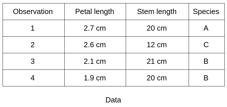
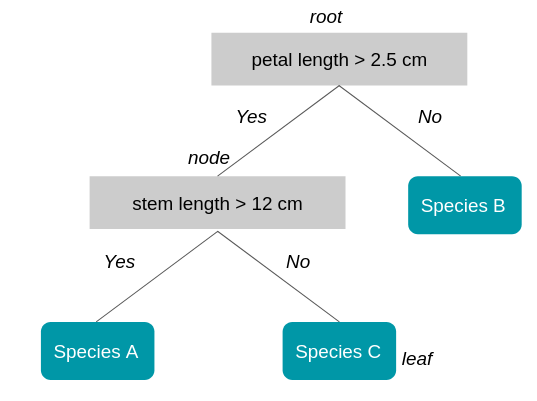
L’arbre a une profondeur de 2 (un noeud plus la racine). La longueur de la pétale est la première mesure qui est utilisée car elle sépare le mieux les 4 observations selon l’appartenance aux classes (ici à la classe B).
B. "Les Forêts Aléatoires"
Comme son nom l’indique l’algorithme des forêts aléatoires se fonde sur les arbres de décisions.Pour mieux comprendre l’intérêt et le fonctionnement de cet algorithme commençons par un exemple :Vous êtes à la recherche d’une bonne destination de voyage pour vos prochaines vacances. Vous demandez à votre meilleur ami son avis. Il vous pose des questions sur vos précédents voyages et vous fait une recommandation.Vous décidez de demander à un groupe d'ami qui vous posent des questions de manière aléatoire. Ils vous font chacun une recommandation. La destination retenue est celle qui a été la plus recommandée par vos amis.Les recommandations faites par votre meilleur ami et le groupe vous paraîtront toutes deux de bons choix de destination. Mais lorsque la première méthode de recommandation marchera très bien pour vous, la deuxième sera plus fiable pour d’autres personnes.Cela vient du fait que votre meilleur ami, qui construit un arbre de décision pour vous donner une recommandation de destination, vous connaît très bien ce qui a fait que l’arbre de décision a sur-appris sur vous (on parle d'overfitting : sur apprentissage).Votre groupe d'ami représente la forêt aléatoire de multiples arbres de décisions et c’est un modèle, lorsqu’il est bien utilisé, évite l’écueil de l’overfitting.
Comment est donc est construite cette forêt?
En voici les principales étapes :
- On prend un nombre X d'observations du jeu de données de départ (avec remise).
- On prend un nombre K des M variables disponibles (features),par exemple : seulement température et densité de population
- On entraîne un arbre de décision sur ce jeu de données.
- On répète les étapes 1. à 4. N fois de sorte à obtenir N arbres.
Pour une nouvelle observation dont on cherche la classe on descend les N arbres. Chaque arbre propose une classe différente. La classe retenue est celle qui est la plus représentée parmi tous les arbres de la forêt. (Vote majoritaire / 'Ensemble' en anglais).
C. Le "Gradient Boosting" / "XG Boost"
La méthode du gradient boosting sert à renforcer un modèle qui produit des prédictions faibles, par exemple un arbre de décision (voir comment juge-t-on la qualité d’un modèle).Nous allons expliquer le principe du gradient boosting avec l’arbre de décision mais cela pourrait être avec un autre modèle.Vous avez une base de données d’individu avec des informations de démographie et des activités passés. Vous avez pour 50% des individus leur age mais l’autre moitié est inconnue.Vous souhaitez obtenir l'âge d'une personne en fonction du ses activités : courses alimentaires, télévision, jardinage, jeux vidéo …Vous choisissez comme modèle un arbre de décision, dans ce cas c’est un arbre de régression car la valeur à prédire est numérique.Votre premier arbre de régression est satisfaisant mais largement perfectible : il prédit par exemple qu’un individu a 19 ans alors qu’en réalité il en a 13, et pour un autre 55 ans au lieu de 68.Le principe du gradient boosting est que vous allez refaire un modèle sur l’écart entre la valeur prédite et la vraie valeur à prédire.AgePrediction Tree 1DifferencePrediction Tree 21319-6156855+1363On va répéter cette étape N fois où N est déterminé en minimisant successivement l’erreur entre la prédiction et la vraie valeur.La méthode pour optimiser est la méthode de descente du gradient que nous n’expliquerons pas ici.Le modèle XG Boost (eXtreme Gradient Boosting) est une des implémentations du gradient boosting fondé par Tianqi Chen et a séduit la communauté de datascientist Kaggle par son efficacité et ses performances. Le publication expliquant l’algorithme se trouve ici.
D. "Les Algorithmes Génétiques"
Comme leur nom l’indique les algorithmes génétiques sont basés sur le processus d’évolution génétique qui a fait de nous qui nous sommes…Plus prosaïquement il sont principalement utilisés lorsqu’on ne dispose pas d’observations de départ et qu’on souhaite plutôt qu’une machine apprenne à apprendre au fur et à mesure de ses essais.Ces algorithmes ne sont pas les plus efficaces pour un problème spécifique mais plutôt pour un ensemble de sous-problèmes (par exemple apprendre l’équilibre et la marche en robotique).Prenons un exemple simple :Nous souhaitons trouver le code d’un coffre fort qui est fait de 15 lettres :“MACHINELEARNING”L’approche en algorithmie génétique sera la suivante :On part d’une population de 10 000 “chromosomes” de 15 lettres chacun. On se dit que le code est un mot ou un ensemble de mots proches.“DEEP-LEARNING”“STATISTICAL-INFERENCE”“INTERFACE-HOMME-MACHINE”etc.Nous allons définir une méthode de reproduction : par exemple combiner le début d’un chromosome avec la fin d’un autre.Ex : “DEEP-LEARNING” + “STATISTICAL-INFERENCE” = “DEEP-INFERENCE”Ensuite nous allons définir une méthode de mutation ce qui permet de faire évoluer une descendance qui est bloquée. Dans notre cas ce pourrait être faire varier une des lettres aléatoirement.Enfin nous définissons un score qui va récompenser telle ou telle descendance de chromosomes. Dans notre cas où le code est caché nous pouvons imaginer un son que ferait le coffre lorsque 80% des lettres sont similaires et qui deviendrait de plus en plus fort à mesure que nous nous approchons du bon code.Notre algorithme génétique va partir de la population initiale et former des chromosomes jusqu’à ce que la solution a été trouvée.
E. Les “Machines à Vecteurs de Support”
Aussi connu sous le nom de “SVM” (Support Vector Machine) cet algorithme sert principalement à des problèmes de classification même si il a été étendu à des problèmes de régression (Drucker et al., 96).Reprenons notre exemple de destinations idéales de vacances. Pour la simplicité de notre exemple considérons seulement 2 variables pour décrire chaque ville : la température et la densité de population. On peut donc représenter les villes en 2 dimensions.Nous représentons par des ronds des villes que vous avez beaucoup aimé visiter et par des carrés celles que vous avez moins apprécié. Lorsque vous considérez de nouvelles villes vous souhaitez savoir de quelle groupe cette ville se rapproche-t-elle le plus.Comme nous le voyons sur le graphique de droite il existe de nombreux plans (des droites lorsque nous n'avons que 2 dimensions) qui sépare les deux groupes.
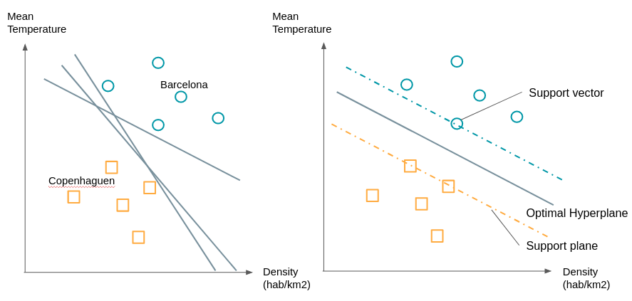
On va choisir la droite qui est à la distance maximale entre les deux groupes. Pour le construire nous voyons déjà que n’avons pas besoin de tous les points, il suffit de prendre les points qui sont à la frontière de leur groupe on appelle ces points ou vecteurs, les vecteurs supports. Les plans passant par ces vecteurs supports sont appelés plans supports. Le plan de séparation sera celui qui sera équidistant des deux plans supports.Que faire si les groupes ne sont pas aussi facilement séparable, par exemple sur une des dimensions des ronds se retrouvent chez les carrés et vice-versa?Nous allons procéder à une transformation de ces points par une fonction pour pouvoir les séparer. Comme dans l’exemple ci-dessous :
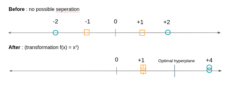
L’algorithme SVM va donc consister à chercher à la fois l’hyperplan optimal ainsi que de minimiser les erreurs de classification.
F. Les “K plus proches voisins”
Pause. Après 5 modèles relativement techniques l’algorithme des K plus proches voisins vous paraîtra comme une formalité. Voici comment il marche :
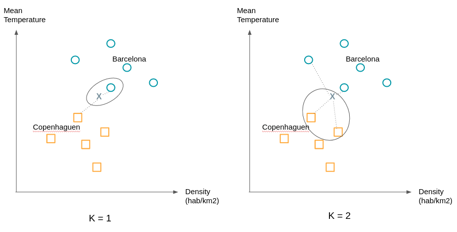
On affecte à une observation la classe de ses K plus proches voisins. “C’est tout?!” me direz vous. Oui c’est tout, seulement comme l’exemple suivant le montre le choix de K peut changer beaucoup de choses.On cherchera donc à essayer différentes valeurs de K pour obtenir la séparation la plus satisfaisante.
G. La "Régression Logistique"
Rappelons pour commencer le principe de la régression linéaire. La régression linéaire est utilisée pour prédire une variable numérique, par exemple le prix du coton en fonction d’autres variables numériques ou binaires : le nombre d’hectares cultivables, la demande en coton de diverses industries etc.Il s’agit de trouver les coefficients a1, a2, … pour avoir la meilleure estimation :Prix du coton = a1 * Nombre d’hectares + a2 * Demande de coton + …La régression logistique est utilisée en classification de la même manière que les algorithmes exposés jusqu’ici. On va reprendre l’exemple de voyages en considérant seulement deux classes : bonne destination (Y=1) et mauvaise destination (Y=0).P(1) : probabilité la ville soit une bonne destination.P(0) : probabilité que la ville soit une mauvaise destination.La ville est représentée par un certain nombre de variables, nous n’allons en considérer que deux : la température et la densité de population.X = (X1 : température, X2 : densité de population)On est donc intéressé de construire une fonction qui nous donne pour une ville X :P(1|X) : probabilité que la destination soit bonne sachant X, ce qui revient à dire probabilité que la ville vérifiant X soit une bonne destination.Nous souhaiterions rattacher cette probabilité à une combinaison linéaire comme une régression linéaire. Seulement la probabilité P(1|X) varie entre 0 et 1 or nous voulons une fonction qui parcourt tout le domaine des nombres réels (de -l’infini à +l’infini).Pour cela nous allons commencer par considérer P(1|X) / (1 – P(1|X)) qui est le ratio entre la probabilité que la destination soit bonne et celle que la destination soit mauvaise. Pour des probabilités fortes ce ratio se rapproche de + l’infini (par exemple une probabilité de 0.99 donne 0.99 / 0.01 = 99) et pour des probabilités faibles il s'approche de 0 : (une probabilité de 0.01 donne 0.01 / 0.99 = 0.0101 ).Nous sommes passé de [0,1] à [0,+infini[. Pour étendre le 'scope' des valeurs possibles à ]-l'infini,0] nous prenons le logarithme népérien de ce ratio.Il en découle que nous cherchons b0,b1,b2, … tels que :ln (P(1|X)/(1 – P(1|X)) = b0 + b1X1 + b2X2La partie droite représente la régression et le logarithme népérien dénote de la partie logistique.L'algorithme de régression logistique va donc trouver les meilleurs coefficients pour minimiser l'erreur entre la prédiction faite pour des destinations visitées et la vraie étiquette (bon, mauvais) donnée.
H. Le "Clustering"
L’apprentissage supervisé vs non supervisé. Vous vous en rappelez?Jusqu’à maintenant nous avons exposé des algorithmes d’apprentissage supervisés. Les classes sont connues et nous souhaitons classifier ou prédire une nouvelle observation. Mais comment faire lorsqu’il n’y a pas de groupe prédéfini? Lorsque vous cherchez justement à trouver des patterns partagés par des groupes d’individus?Par leur apprentissage non supervisé les algorithmes de clustering remplissent ce rôle.Prenons l’exemple d’une entreprise qui a commencé sa transformation digitale. Elle dispose de nouveaux canaux de vente et de communication à travers son site et une ou plusieurs applications mobiles associées. Dans le passé elle s’adressait à ses clients en fonction de données démographiques et son historique d’achat. Mais comment exploiter les données de navigation de ses clients? Le comportement en ligne correspond-t-il aux segments de clientèle classique?Ces questions peuvent motiver l’utilisation du clustering pour voir si des grandes tendances se dégagent. Cela permet d’infirmer ou de confirmer des intuitions métier que vous pouvez avoir.Il existe de nombreux algorithmes de clustering (clustering hiérarchique, k-means, DBSCAN, ...). L’un des plus utilisés est l’algorithme k-means. Nous allons en expliquer le fonctionnement simplement :Même si nous ne savons pas comment seront constitués les clusters l’algorithme k-means impose de donner le nombre de clusters attendus. Des techniques existent pour trouver le nombre optimal de clusters.Considérons l’exemple des villes. Notre jeu de donnée possède 2 variables, on se place donc en 2 dimensions. Après une première étude nous nous attendons à avoir 2 clusters. Nous commençons par placer au hasard deux points; ils représentent nos ‘means’ de départ. Nous associons au mêmes clusters les observations les plus proches de ces means. Ensuite nous calculons la moyenne des observations de chaque cluster et déplaçons le means à la position calculée. Nous ré-affectons les observations au means le plus proche et ainsi de suite.
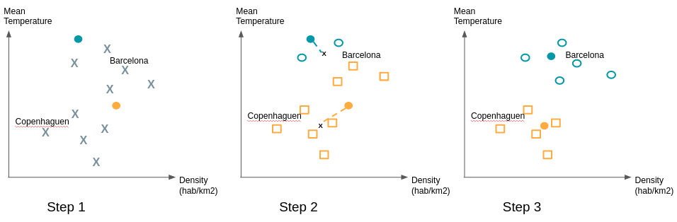
Pour s’assurer de la stabilité des groupes trouvés il est recommandé de recommencer de multiples fois le tirage des ‘means’ initiaux car certains tirages initiaux peuvent donner une configuration différente de la large majorité des cas.
3. Facteurs de pertinence et de qualité des algorithmes de Machine Learning
Les algorithmes de machine learning sont évalués sur la base de leur capacité à classifier ou prédire de manière correcte à la fois sur les observations qui ont servi à entraîner le modèle (jeu d’entraînement et de test) mais aussi et surtout sur des observations dont on connaît l’étiquette ou la valeur et qui n’ont pas été utilisées dans l’élaboration du modèle (jeu de validation).Bien classifier sous-entend à la fois placer les observations dans le bon groupe et à la fois ne pas en placer dans des mauvais groupes.La métrique choisie peut varier en fonction de l’intention de l’algorithme et de son usage métier.Plusieurs facteurs liés aux données peuvent jouer fortement sur la qualité des algorithmes. En voici les principaux :
A. Le nombre d'observations
Moins il y a d'observations plus l'analyse est difficile. Mais plus il y en a, plus le besoin de mémoire informatique est élevé et plus longue est l'analyse).
B. Le nombre et qualité des attributs décrivant ces observations
- La distance entre deux variables numériques (prix, taille, poids, intensité lumineuse, intensité de bruit, etc) est facile à établir.
- Celle entre deux attributs catégoriels (couleur, beauté, utilité…) est plus délicate.
C. Le pourcentage de données renseignées et manquantes
D. Le « bruit »
Le nombre et la « localisation » des valeurs douteuses (erreurs potentielles, valeurs aberrantes…) ou naturellement non-conformes au pattern de distribution générale des « exemples » sur leur espace de distribution impacteront sur la qualité de l'analyse.
Conclusion
Nous avons vu que les algorithmes de machine learning servaient à deux choses : classifier et prédire et qu’ils se divisaient en algorithmes supervisés et non supervisés. Il existe de nombreux algorithmes possibles, nous en avons parcouru 8 d’entre eux dont la régression logistique et les forêts aléatoires pour classifier une observation et le clustering pour faire émerger des groupes homogènes à partir des données. Nous avons également vu que la valeur d’un algorithme dépendait de la fonction coût ou perte associée mais que son pouvoir prédictif dépendait de plusieurs facteurs liés à la qualité et le volume de données.J’espère que cet article vous a donné des éléments de compréhension sur ce qu’on appelle le "Machine Learning". N’hésitez pas à utiliser la partie commentaire pour me faire un retour sur des aspects que vous souhaiteriez clarifier ou approfondir.
Auteur
Gaël BonnardotCofounder and CTO at DatakeenChez Datakeen nous cherchons à simplifier l'utilisation et la compréhension des nouvelles techniques algorithmiques par les fonctions métier de toutes les industries.
À lire également
- 3 Deep Learning Architectures explained in Human Language
- Key Successes of Deep Learning and Machine Learning in production
Sources
- http://blog.kaggle.com/2017/01/23/a-kaggle-master-explains-gradient-boosting/
- http://dataaspirant.com/2017/05/22/random-forest-algorithm-machine-learing/
- https://burakkanber.com/blog/machine-learning-genetic-algorithms-part-1-javascript/
- http://docs.opencv.org/3.0-beta/doc/py_tutorials/py_ml/py_svm/py_svm_basics/py_svm_basics.html#svm-understanding
- https://fr.wikipedia.org/wiki/Apprentissage_automatique
Continuer la lecture


Prêt à en voir plus ?
Une nouvelle façon de gérer la vérification d’identité, plus simple et plus sûre.